

Deep Dive into Convolutional Neural Networks, Part 1:
A Beginner's Guide to Convolutional Neural Network Layers


Table of contents
Introduction
Most models used in modern-day computer vision tasks like object detection, generative computer vision, object recognition, and so on all have their backbone architecture in convolutional neural networks (CNN).
A convolutional neural network is a deep neural network used in computer vision to extract image features. A convolutional neural network architecture comprises many interconnected layers, including convolution, pooling, and fully-connected layers.
This series works towards explaining the working principles of implementing a computer vision project. The different parts of the series would break down the key concepts of convolutional neural networks. This article aims to explain the crucial layers present in the CNN architecture.
For an easy grasp of this article, the reader must have a basic knowledge of the following:
Python Programming
Neural Networks
Image Processing
If you are a computer vision newbie, machine learning researcher, or data scientist looking to understand the basics of convolutional neural networks, this article is a perfect start for you.
In the coming sections of this article, there will be explanations of these layers. By the end of the article, you will understand the key layers of CNN's architecture.
Convolutional Layer
The convolutional layer is the fundamental layer in CNN architecture. It extracts meaningful features from an input image. This layer carries out an operation known as "convolution" on the image.
Convolution involves multiplying two functions to produce a third function that expresses how the shape of one function affects the other. When an input image passes through the convolutional layer, the convolution operation occurs between the image and a filter to produce a feature map. A filter is the smallest version of an image made up of learnable weight values.
The filter slides across the input image, computing the element-wise product and the sum of the overlapping regions. This operation repeats across the entire picture to get a feature map.

As you can see in the image above, the convolution operation occurs between the filter and the region covered by the filter. or this operation, the formula gives the pixel value for the new feature matrix
Sliding the filter by any number of strides gives the other pixel values for the feature matrix. The formula below calculates the shape of the feature map produced:
$$H = [(h - F + 2P) / S]+1$$
Parameters
CNN utilizes a convolutional layer to capture spatial patterns and hierarchical representations in the image. Spatial Patterns and hierarchical representations involve edges, corners, textures, etc. Regardless of their positions or scales in an image, CNN recognizes objects or patterns with the help of the convolutional layer. We term this role "spatial invariance".
Implementation of Convolutional Layer with Tensorflow
To build a CNN architecture with the TensorFlow package, we use the CONV2D function present in the package. This function takes the following parameters:
Number of Filters,
Filter Shape,
Activation Function,
Padding,
Strides and
Input Shape.
The syntax represents the convolutional layer
import tensorflow as tf    # Importing tensorflow model.

# Syntax for the convolutional layer
tf.keras.layers.Conv2D(num_filters, filter_shape, activation, padding, strides, input_shape)
The number of filters in the convolutional layer depends on the number of neurons since each neuron performs a different convolution on the input image. The activation function present is to introduce non-linearity into the layer.
Without the activation functions, CNN can only learn linear relationships. The activation function enables it to learn complex and non-linear relationships. The most common activation functions in CNN include softmax, ReLU, and sigmoid.
During the convolution operation, the filter slides over the input image by a certain number of pixels. The number of pixels the filter slides over is known as the stride.
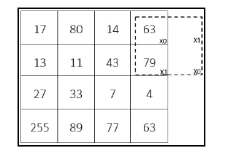
The image below shows the filter sliding over the input image with a stride of two. This means that the filter moves two pixels to the next region.

The filter goes both sideways and downward on the input image. Sometimes, the filter does not fit the input matrix after sliding it over, like in the image below. In this situation, padding preserves the input image's spatial dimension.
Padding introduces extra pixels around the sides of the input feature map before convolution. There are two padding methods: "Same Padding" and "Valid Padding".
Same-Padding adds empty pixels to the sides of the input feature map so that it has the same shape as the output feature map. Zero padding, the most common, adds pixels with values of 0 to the filter's edge. The image below describes how it carries out this padding method.

To derive the number of pixels the padding would fill depending on the filter size used in the convolutional layer,
$$padding = (F-1) / 2$$
If the convolutional layer takes in a filter size of (5, 5), this method pads two pixels based on the formula. To assign zero padding to a convolutional layer, the padding parameter is set to using the syntax padding = "same".
In the case of valid padding, no padding is added to the pixels; the filter goes over the valid pixels alone. No form of padding occurs on the sides of the input feature map. The padding parameter is set to “valid” with the syntax as padding = "valid".
Due to this, the formula for the output feature map changes since padding becomes zero in the convolutional layer. The new formula becomes
$$H = [(h - F) / S] + 1$$
Parameters
When the convolutional layer receives the parameters explained above, it performs the convolution operation which produces the output feature maps that can be further fed to other convolutional layers or the pooling layer.
The coming section will explain the meaning of the pooling layers, their roles, and their implementation using TensorFlow.
Pooling Layers
Due to the computational space on which the convolutional layer operates, the pooling layer reduces the dimensions of the feature maps. It does this while keeping the important features in the image.
The pooling layer changes the height and width of the feature maps but does not change their depth. Translational invariance is the term used to describe these characteristics. The pooling layer performs an operation known as the downsampling or subsampling operation.
The pooling operation is classified into various types, such as the max pooling operation, the average pooling operation, and the sum pooling operation. Like the convolution operation, a filter matrix slides over the input feature map to reduce the image dimension, depending on the operation selected.
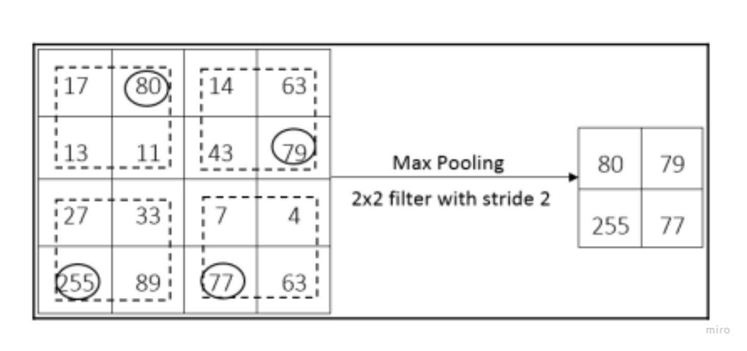
For the max pooling operation, the most value from the region covered by the filter matrix is selected. As the image below portrays, the stride determines the region over which the max pooling operation occurs.
In the case of the sum pooling operation, the total sum of the individual pixel values in the region is calculated. This sum represents the new pixel of the output feature map.
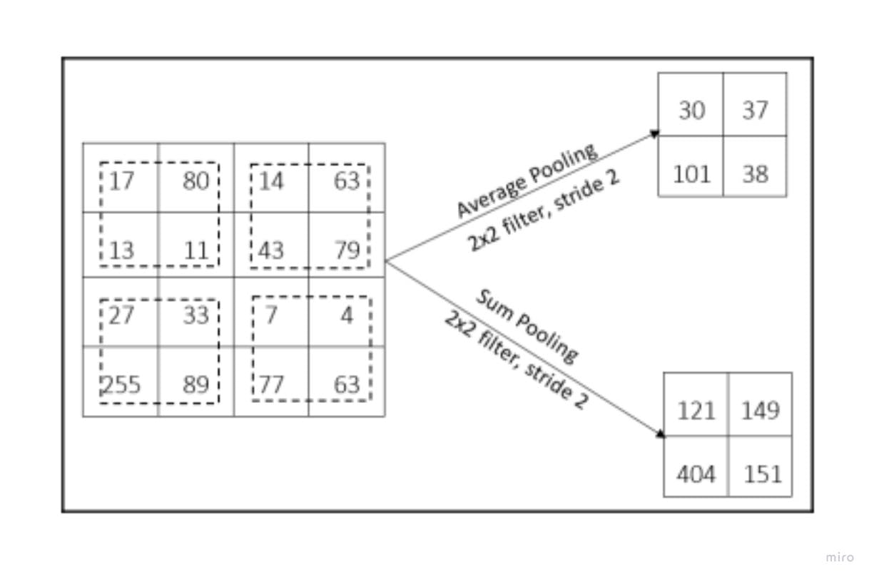
The average pooling operation takes the average of the region as the new pixel. Depending on the size of the filter, the formula used to calculate the average is:
$$average = [a+b+c+.....+d] / n$$
Parameters
It is necessary to understand how this operation can be implemented using TensorFlow. This topic will be further discussed in the sub-section.
Implementing the Pooling Operation with Tensorflow.
Depending on one's choice, Tensorflow offers a class that allows users to use different kinds of pooling operations. This article points out the syntax for the pooling operation explained above.
All three of the pooling operations take one parameter, which is the pooling shape. The pooling shape is the size of the filter that slides over the feature map.
The syntax for each of the operations is
# Max Pooling Layer
tf.keras.layers.MaxPooling2D(pooling_shape)

# Average Pooling Layer
tf.keras.layers.AvgPooling2D(pooling_shape)

# Sum Pooling Layer
tf.keras.layers.SumPooling2D(pooling_shape)
The convolutional layer and pooling layer explained above are of great importance when it comes to extracting features from the image. When working with classification tasks in images, the extracted features can only be classified after they are passed into the fully-connected layer. The next section explains the fully-connected layer to a great extent.
Fully-Connected Layer
Understanding how classification tasks are performed with neural networks will give the reader a basic knowledge of the fully-connected layers.
The fully-connected layer consists of the flatten layer and the dense layer. The extracted feature maps from the final convolutional or pooling layer remain a two-dimensional array. The task of the flatten layer is to convert the extracted feature map into a one-dimensional array.
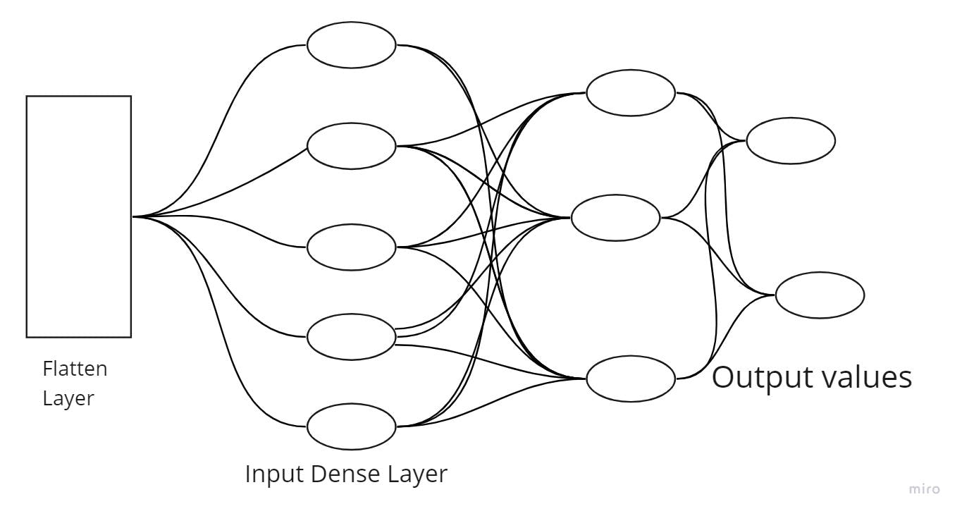
The one-dimensional array is fed into the dense layer, which performs the classification task. The dense layers are stacked so that the low-level and high-level features are derived for classification. Three types of dense layers are necessary parts of the fully-connected layer: input, hidden, and output. Each of these layers is present to improve the classification accuracy of the model.
Implementing a Fully-Connected Layer
The fully-connected layer can be easily implemented using TensorFlow. Although the flatten layer function takes no parameters, the dense layer takes several parameters.
The main parameters the dense layer takes into account are units and the activation function. The unit parameter defines the size of the output from the dense layer. As explained in the Implementation of Convolutional layer section, the Dense layer also takes in the activation function and performs the same task.
These syntaxes execute the roles of the flatten and dense layers.
# Flatten Layer
tf.keras.layers.Flatten()
# Dense Layer
tf.keras.layers.Dense(units, activation)
The dense layer can be repeated a couple of times to improve the model's accuracy in classifying the image.
With each of the layers in the convolutional neural network explained above, creating a simple CNN model gives a proper view of how the architecture of an image classification model is built. The next section emphasizes this task.
Building a Simple Convolutional Neural Network Architecture.
A convolutional neural network architecture is the arrangement of the layers. Various state-of-the-art models are built by stacking these different layers together in a spectacular way.
The manner of arrangement differs for various models. To come up with a simple CNN architecture that is employable in an image recognition task, one can use the Sequential API from Tensorflow.
The model will contain five convolutional layers and four max pooling layers. Then, the extracted feature maps are flattened using the Flatten layer. The dense layer performs the recognition task and outputs the final class of the image. Below is a code that builds this model.
# importing Python libraries.
from tensorflow.keras import Sequential, layers

# the Sequential model is defined
model = Sequential([
    layers.Conv2D(16, (3,3), activation= 'relu', input_shape =(150, 150, 3)),
    layers.MaxPooling2D(2,2),
    layers.Conv2D(32, (3,3), activation='relu', padding=same, stride=2),
    layers.MaxPooling2D(2,2),
    layers.Conv2D(64, (3,3), activation='relu'),
    layers.MaxPooling2D(2,2),
    layers.Conv2D(64, (3,3), activation='relu', padding=same, stride=2),
    layers.MaxPooling2D(2,2),
    layers.Conv2D(64, (3,3), activation='relu'),
    layers.Flatten(),
    layers.Dense(512, activation='relu'),
    layers.Dense(256, activation='relu')
    layers.Dense(1,activation= 'sigmoid'),
])
The layers in the model show how the CNN layers can be stacked and how the parameters are set in each layer. When working on an image recognition project, this model can serve as a guide for building the reader’s model. The model can be further trained to improve the accuracy score.
Conclusion
Basic knowledge of convolutional neural network layers helps the reader understand more complex and complicated models. The reader can now work on an image classification task without much difficulty.
Although, not all the convolutional neural network layers are touched on in this article. Other layers, like the dropout, batch normalization, etc., are easy to comprehend with this knowledge.
This series would carry on to explain how to deal with data for an image classification task.
Reference
You are encouraged to source for more understanding on this topic. Some resources used for this article are provided below.
Hands-on Deep Learning Algorithms with Python by Sudharsan Ravichandran: Demystifying Convolutional Network, Page 216.
Hands-on Machine Learning with Scikit-Learn, Keras & Tensorflow: Deep Computer Vision Using Convolutional Neural Networks, Page 457.
Deep Learning with Python Second Edition: Introduction to Deep Learning for Computer Vision, Page 201.
Convolutional Neural Networks Explained — How To Successfully Classify Images in Python